Whether you're a beginner stepping into programming or a data enthusiast diving into automation, Python is a great language to start with. In this post, we’ll explore various ways to install Python, both locally on your computer and through online platforms, so you can choose the one that works best for you.
Installing Python Locally
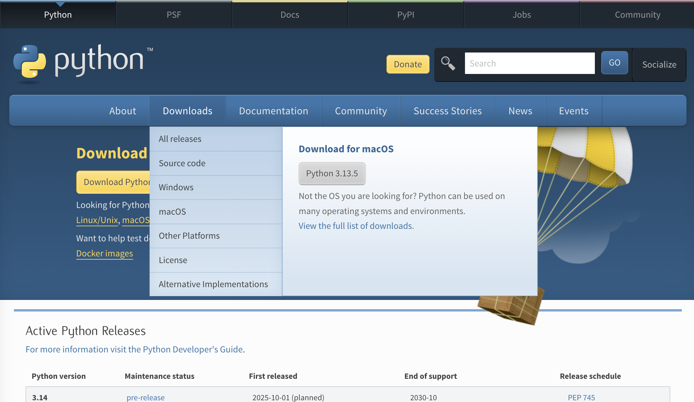
Let's explore steps to install Python on various Operating Systems. Let's start by downloading the latest package by either hovering on Downloads and downloading package or by visting https://www.python.org/downloads/
Installing python on Windows
Start by downloading latest .exe
Once downloaded, double click on it to open installer
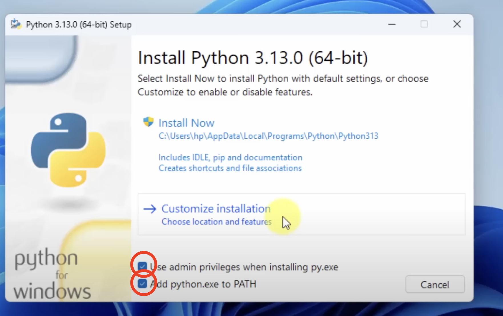
After checking both boxes, click on Customize Installation and checkmark everything
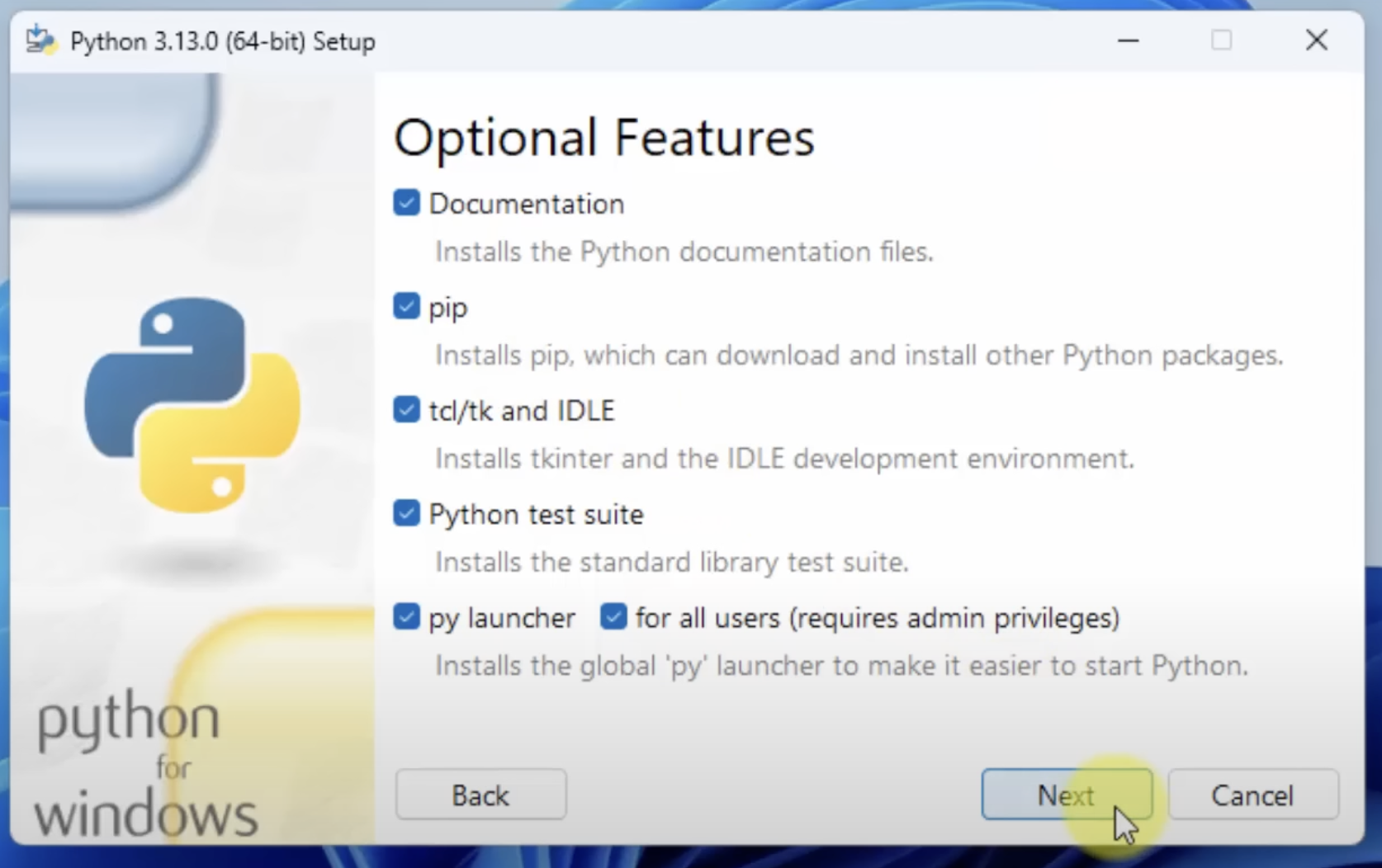
click on Next , then checkmark as per following screenshots
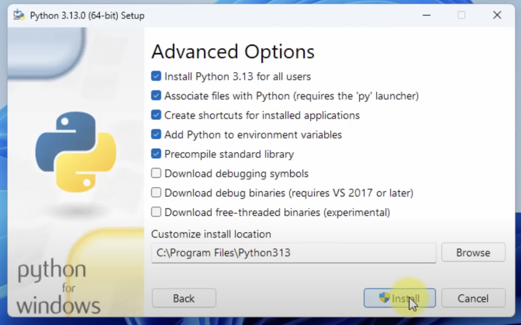
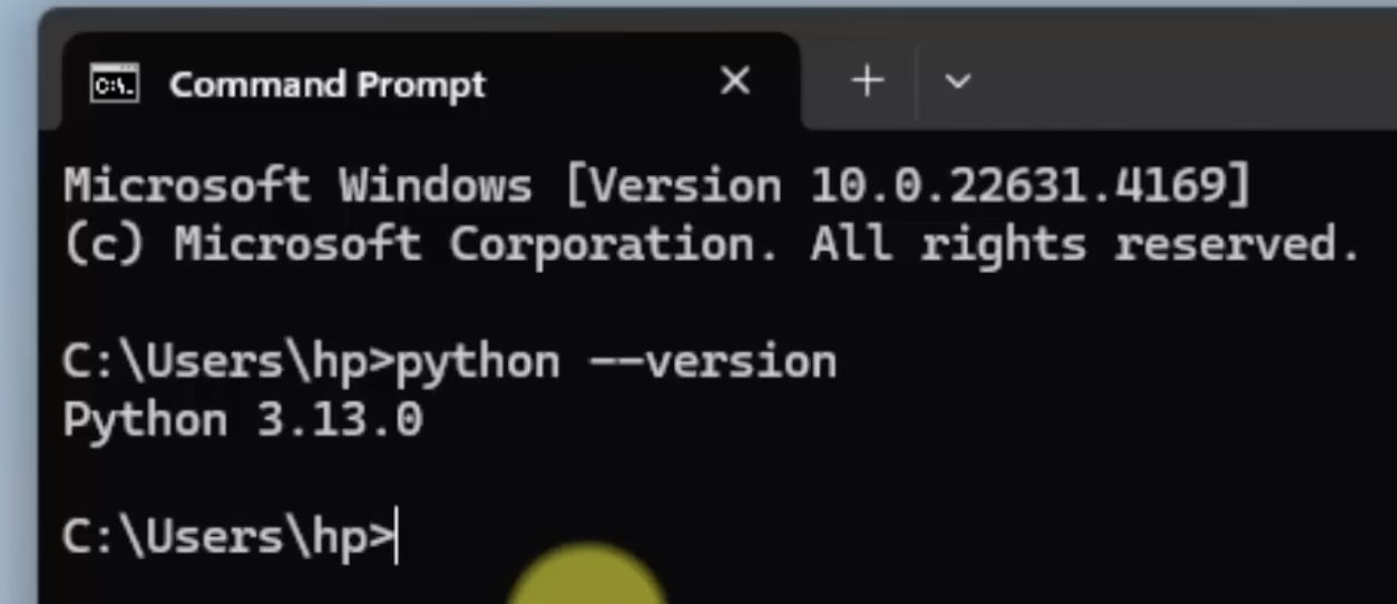
and then click on Install. After installation is done, you can open Command Prompt and confirm if installation is done by typing
python --version
and if you see following result, it means your installation is done !
Installing python on Ubuntu
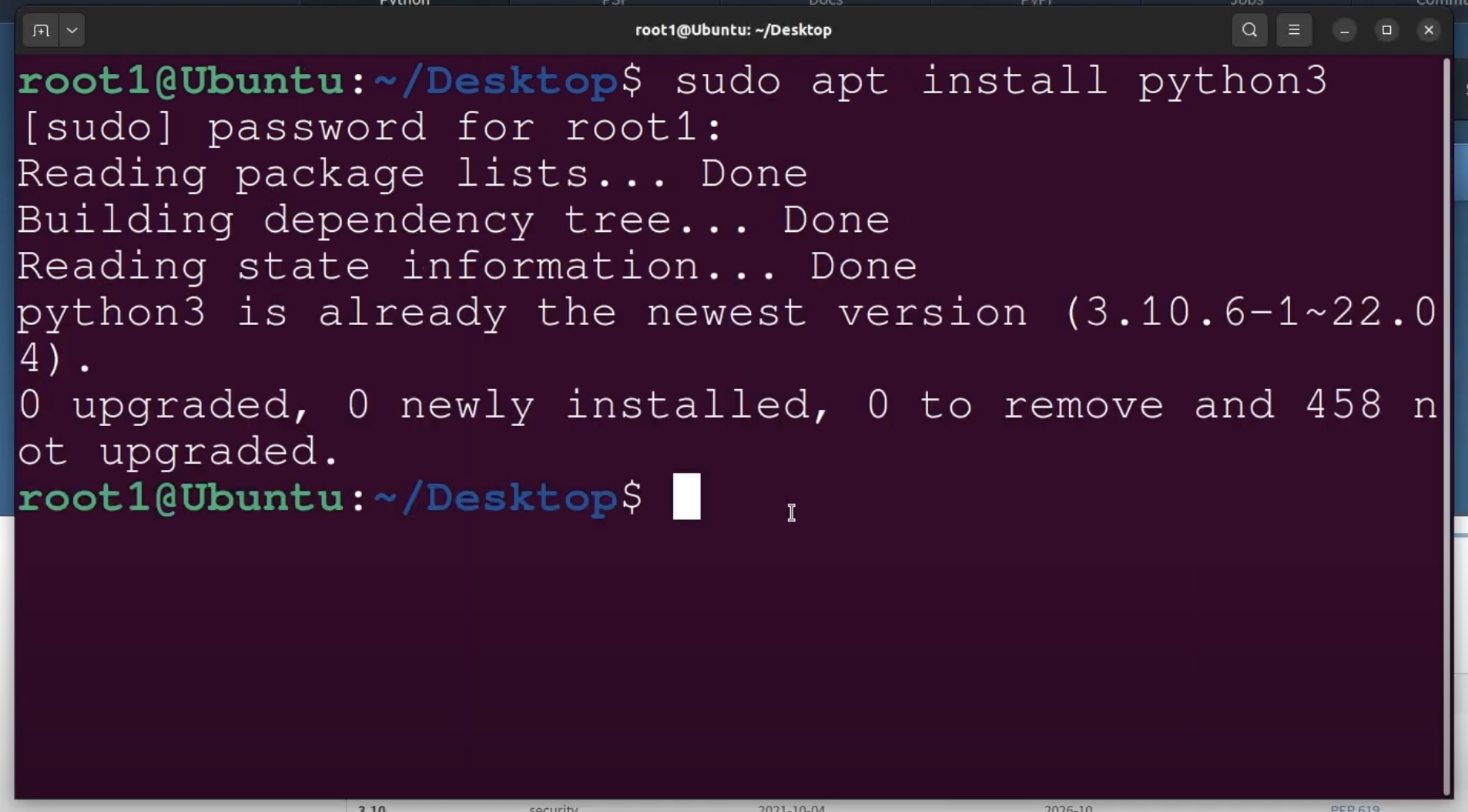
Open terminal and enter following command
sudo apt install python3
enter your password.
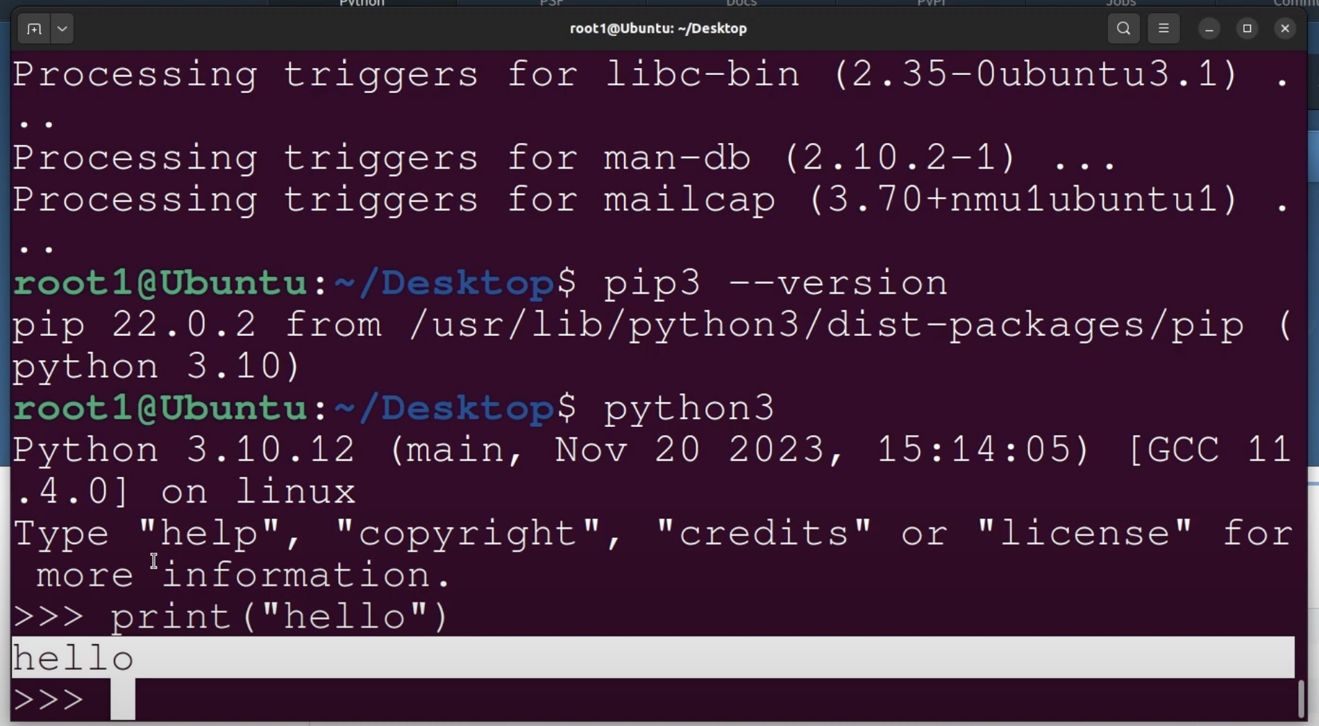
after installing python3, we also need to install pip which manages the packages in python. To install pip, execute following command
sudo apt install python3-pip
You can check if the installations are done correctly by typing
python3 --version #to check python installation
pip3 --version # to check pip installation
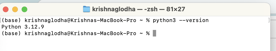
Installing python on MacOS X
Installing Python on MacOS X is similar to Windows, you can download the installer and following the commands
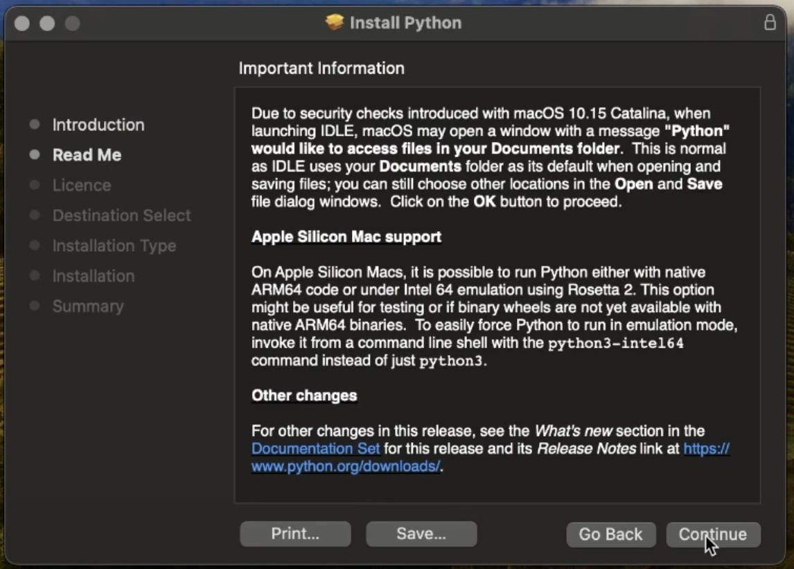
once the installation is done, check on terminal
Hosted Python Environments (No Installation Required!)
If you don’t want to install anything yet, you can run Python in the cloud. Ideal for learning or quick testing.
1. Google Colab
-
Free, cloud-based Jupyter notebooks with access to GPU
-
Great for data science and ML
2. Replit
-
URL: replit.com
-
Supports Python and many other languages
-
Includes a file manager, debugger, and terminal
3. Jupyter Notebook (via Binder)
-
URL: mybinder.org
-
Turn any GitHub repo into an executable notebook