Pytorch workflows¶

Day 4¶

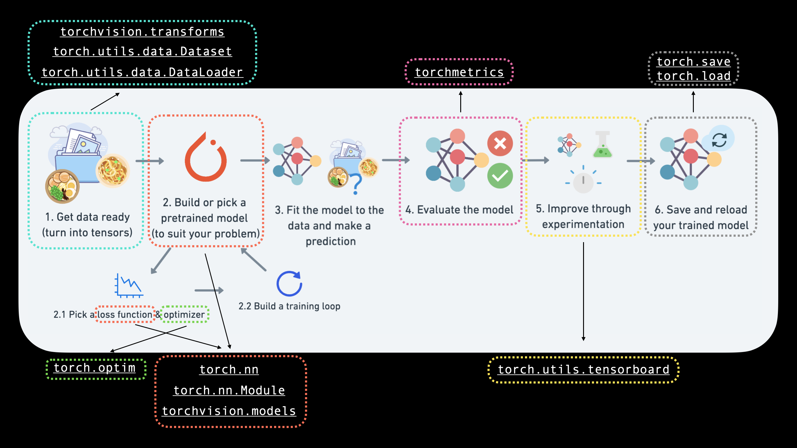
AS per the image the general flow for any AI problem can be written in following steps

1. Data Preparation and loading
2. Building model
3. Fitting the model to data (training)
4. Making predication adn evaluating model (inference)
5. Saving and loading model
6. Putting everything together for deployment

In [30]:

import torch
from torch import nn # nn (neural network) are all the building blocks available for us to use from pytorch

import torch from torch import nn # nn (neural network) are all the building blocks available for us to use from pytorch

At this point it is important to clear fundamentals of nueral networks. I found following video very useful

In [31]:

import matplotlib.pyplot as plt # we need matplotlib for visualisation

import matplotlib.pyplot as plt # we need matplotlib for visualisation

Loading Data and Preparing¶

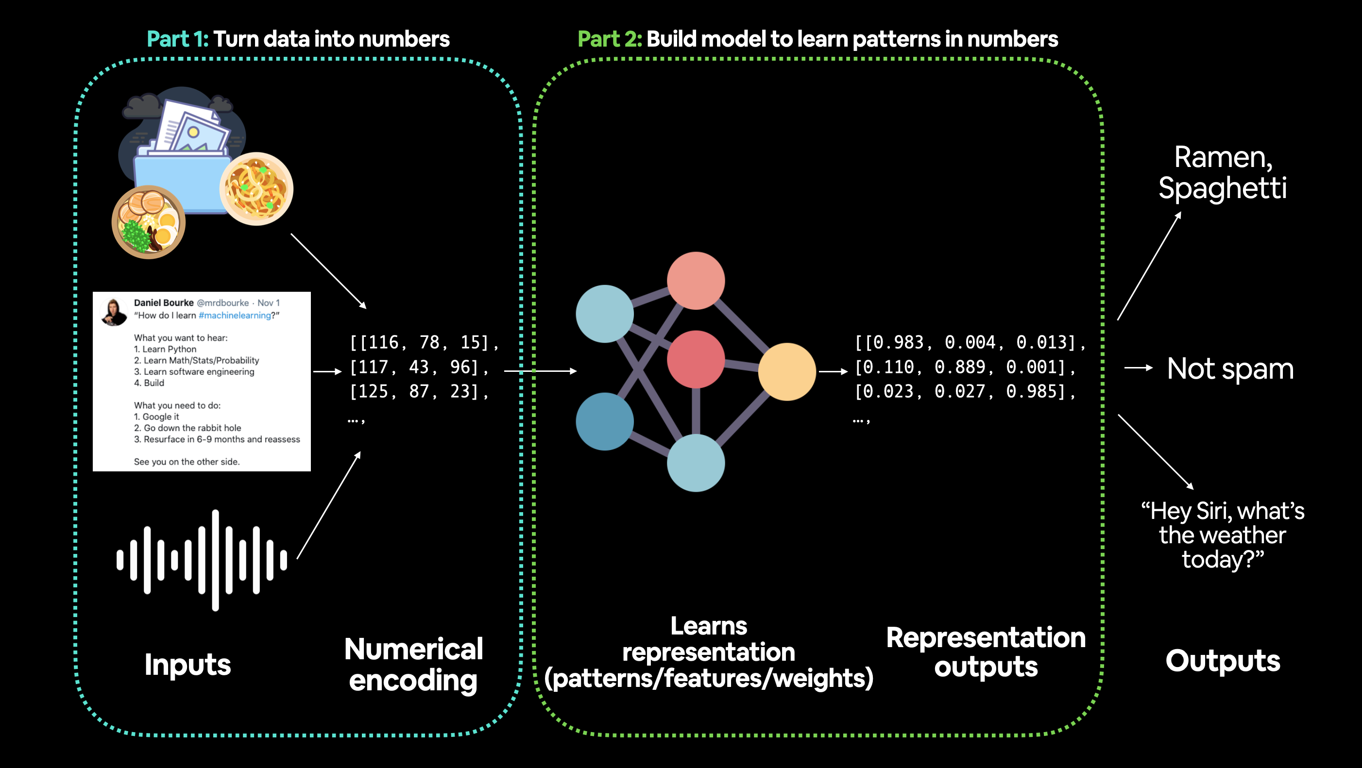
Any data can be used in ML algorithm ( Images, Videos, Texts, Files, etc.). Thus data preparing can be divided in 2 parts

1. converting input data into numerical representation
2. Build model to figure out patterns in that representation

Let's start by learning linear regression. Again, before jumping in code and deciding to give up :P , checkout concept

hindi

english

In [32]:

weight = 0.3 # slope 
bias = 0.4 # value of Y when X is 0 

# creating tensors for Y and X

range_start = 10
range_end = 20
step = 0.03

X = torch.arange(range_start, range_end, step).unsqueeze(1) # we have added unsqueeze to add extra dimension to tensor

Y = weight * X + bias

X[:3],Y[:3]

weight = 0.3 # slope bias = 0.4 # value of Y when X is 0 # creating tensors for Y and X range_start = 10 range_end = 20 step = 0.03 X = torch.arange(range_start, range_end, step).unsqueeze(1) # we have added unsqueeze to add extra dimension to tensor Y = weight * X + bias X[:3],Y[:3]

Out[32]:

(tensor([[10.0000],
         [10.0300],
         [10.0600]]),
 tensor([[3.4000],
         [3.4090],
         [3.4180]]))

As per the arrangement above we can see that as the value of element in X changes, corresponding value is generated in Y based on weight ( slope ) and bias ( initial value ).

We need to split the data into training and testing dataset. General rule of thumb would be to split data as follows

• Training = 60~80%
• Validation = 10~20% ( Optional )
• Testing = 10~20%

In [33]:

# For our data set total dataset we have is 
print(f"count of data in X is {len(X)}")
print(f"count of data in Y is {len(Y)}")

# For our data set total dataset we have is print(f"count of data in X is {len(X)}") print(f"count of data in Y is {len(Y)}")

count of data in X is 334
count of data in Y is 334

In [34]:

# count of training sample
count_X = int(0.8*len(X))
count_Y = int(0.8*len(Y))
# make training set ~ training split
train_X = X[:count_X]
train_Y = Y[:count_Y]
# make testing set ~ testing split
test_x = X[count_X:]
test_y = Y[count_Y:]

# count of training sample count_X = int(0.8*len(X)) count_Y = int(0.8*len(Y)) # make training set ~ training split train_X = X[:count_X] train_Y = Y[:count_Y] # make testing set ~ testing split test_x = X[count_X:] test_y = Y[count_Y:]

In [35]:

# display train_X, train_Y on matplotlib plot
plt.plot(train_X, train_Y, 'ro')
plt.show()

# display train_X, train_Y on matplotlib plot plt.plot(train_X, train_Y, 'ro') plt.show()

Building Model¶

Let's start by creating linear regression model in pytorch.

To do this we'll be extending nn.Module , which is a base class for all inbuilt ot custom classes we'll be building.

Concepts to learn

• nn.Parameter - Just like how we add parameters to any function in python, nn.Parameter allows us to send tensor as paramter for module classes. The reason why we use nn.parameter to assign tensor is because then we can access it via Class paramters.
• Gradient descend

Essentials for building models¶

• torch.nn = which are hte building blocks of various Neural Networks (Computational Graphs)
• torch.nn.Module = The base class for all Neural Networks. We can make our own subclass of this by writing forward() function
• torch.nn.Parameter = They are used to define attributes in the Modules
• torch.optim = These is a package implementing various optimization algorithms.

In [36]:

# Class for Linear Regression
class LinearRegressionModel(nn.Module):
    # required syntaxt by python
    def __init__(self):
        super().__init__()
        self.weights = nn.Parameter(torch.randn(1,requires_grad=True, dtype=torch.float))
        self.bias = nn.Parameter(torch.randn(1, requires_grad=True, dtype=torch.float))

    # forward method to define computation
    def forward(self, x:torch.Tensor) -> torch.Tensor: # x is input tensor
        return self.weights * x + self.bias  # mx + c

# Class for Linear Regression class LinearRegressionModel(nn.Module): # required syntaxt by python def __init__(self): super().__init__() self.weights = nn.Parameter(torch.randn(1,requires_grad=True, dtype=torch.float)) self.bias = nn.Parameter(torch.randn(1, requires_grad=True, dtype=torch.float)) # forward method to define computation def forward(self, x:torch.Tensor) -> torch.Tensor: # x is input tensor return self.weights * x + self.bias # mx + c

In [17]:

# let's create instance of our model
torch.manual_seed(774)
model_0 = LinearRegressionModel()

# let's create instance of our model torch.manual_seed(774) model_0 = LinearRegressionModel()

In [22]:

# Let's checkout parameters
print(list(model_0.parameters()))

print('---')
# let's print parameters with name 
print(model_0.state_dict())

## Reason we got Tensor with some value in it is because while creating Class, we are using `torch.randn`

# Let's checkout parameters print(list(model_0.parameters())) print('---') # let's print parameters with name print(model_0.state_dict()) ## Reason we got Tensor with some value in it is because while creating Class, we are using `torch.randn`

[Parameter containing:
tensor([0.3003], requires_grad=True), Parameter containing:
tensor([0.3924], requires_grad=True)]
---
OrderedDict([('weights', tensor([0.3003])), ('bias', tensor([0.3924]))])

---